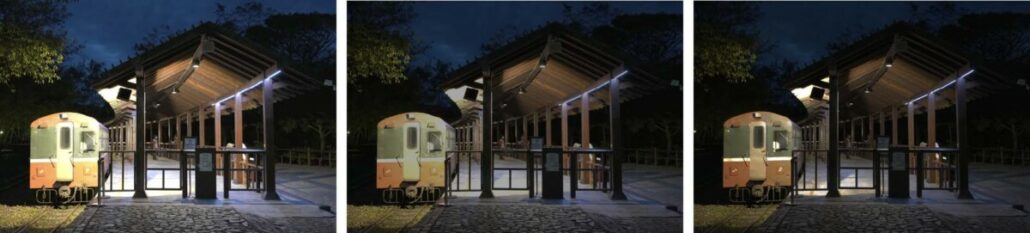
Fig. 1 (Left) original image (Middle) result image of adjusting the brightness directly (Right) result image of adjusting the exposure on our reconstructed radiance map.

Nowadays, more and more people like to take pictures with smartphones and post on social media to share beautiful photos with their friends. Usually, they do some image editing before they post, such as applying filters, adjusting color warmth, saturation or contrast. However, there is one thing they can never change unless they go back to the place where they took the photo and shoot again, i.e., exposure, a parameter that is fixed forever after you click the shutter button. Although it is possible to simulate exposure change effects by adjusting the picture’s brightness, like the middle image of Fig.1, existing tools do not allow us to recover the details of an over-exposed or under-exposed region due to the limitations of the camera sensor.  We propose to solve this issue by reconstructing the radiance map for the image and using GANs to predict the ill-exposed regions. See the right image of Fig.1 as an example. We can recover the missing details on the train (see Fig. 2 to get a closer look), making the result more realistic. With our technique, users can adjust the exposure parameter to have the image they want without going back to the place and taking it again. We will focus on building the model to reconstruct the radiance map in the following and provide more results.

 

Background

We first explain the jargon to provide background knowledge to the readers. If you are  familiar with them, feel free to skip this section.

• Radiance map: a map that records the true luminance value of the scene. The channel value of a pixel is usually represented by a real number with a large range. We also name it HDR image in this article at times. 
• HDR image: abbreviation of High Dynamic Range image, identical to the term radiance map in the article. 
• LDR image:  abbreviation of Low Dynamic Range image. It is the conventional image, where the channel value of a pixel is represented by an 8-bit number, ranging from 0 to 255. LDR images can be generated by tone mapping from the HDR image and displayed on normal screens. 
• Tone mapping: the process of mapping an HDR (high dynamic range) image to an LDR (low dynamic range) image which can be displayed.

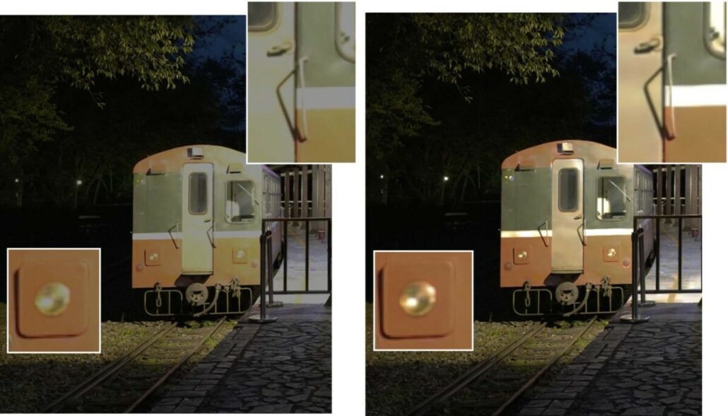
Fig. 2 A closer look of the difference between (Left) naive brightness adjustment and (Right) our result.

Our Method

In the camera, the sensor array records pixels’ values according to the scene radiance and the exposure setting. Due to the limited range of the sensor, excessive values are clipped. To better human perception, the values are nonlinearly mapped using the CRF (camera response function). Finally, the values are quantized and stored into an 8-bit number. The processes of clipping, nonlinear mapping, and quantization all lead to information loss. 

Inspired by [1], we reconstruct the HDR image by reversing the camera pipeline. Starting from an input LDR image, we inverse the CRF by simply applying a square-root mapping. At the next step, we let the model predict values of over-exposed regions, which are clipped by the camera to reconstruct the HDR image. Two key features differentiate our method from other HDR reconstruction methods [1,4,5,6]. The first one is the architecture; unlike Liu et al. [1], which uses an encoder-decoder network to predict values, we treat value prediction in the over-exposed region as an inpainting task in the linear space because GANs can generate better and more realistic results. The second one is that we predict relative luminance instead of absolute luminance. Our goal is to get correct brightness changes and details when applying different exposure parameters, so it is more important to get relatively correct values.

Also, predicting relative luminance is more manageable than predicting the absolute one. About the architecture, we use the U-Net with gated convolution [2] layers (Fig. 3). We also add skip connections, as our experiment shows that they offer clearer and more realistic results. For the discriminator (Fig. 4), we use SN-PatchGAN [2]. Instead of passing the predicted HDR image to the discriminator, we pass the LDR image as the input of the discriminator network. Our experiment shows that passing an image in the linear space as input will cause artifacts in the results. We tone-map an HDR image to an LDR image by directly clipping the value to [0-1] and applying a naive CRF to simulate digital cameras.  

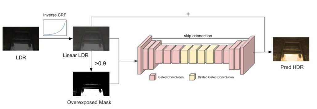
Fig. 3 Our generator model.

 

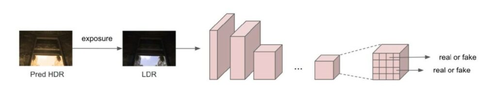
Fig. 4 Our discriminator model (SN-PatchGAN in [2]).

 

Dataset

Data cleaning

We use the dataset provided by singleHDR [1]. However, we found that images of the dataset record relative luminance. Thus the same scene can have different value scales. The scale differences could confuse the model and get worse results. For addressing that issue, we perform data normalization before training to make most pixels (95% in our case) range within [0-1]. This way,all values are of a similar scale so that the model can predict more stably.

Data augmentation

For previous methods [4, 5, 6] that predict absolute luminance, the data augmentation process generates LDR images by applying different CRF curves to the same HDR image to create additional data pairs. They expect those LDR images to be reconstructed into the same HDR image, so they generate data pairs like [GT-HDR, LDR-ev+3], [GT_HDR, LDR-ev+0], [GT_HDR, LDR-ev-3]. For our method, which predicts relative luminance, our data augmentation process generates LDR images by applying different CRF curves to the same HDR image as others do. However, we will create data pairs [GT-HDR-ev+3, LDR-ev+3], [GT-HDR-ev0, LDR-ev0], [GT-HDR-ev-3, LDR-ev-3] (Fig. 5) because we predict relative luminance instead of absolute luminance.

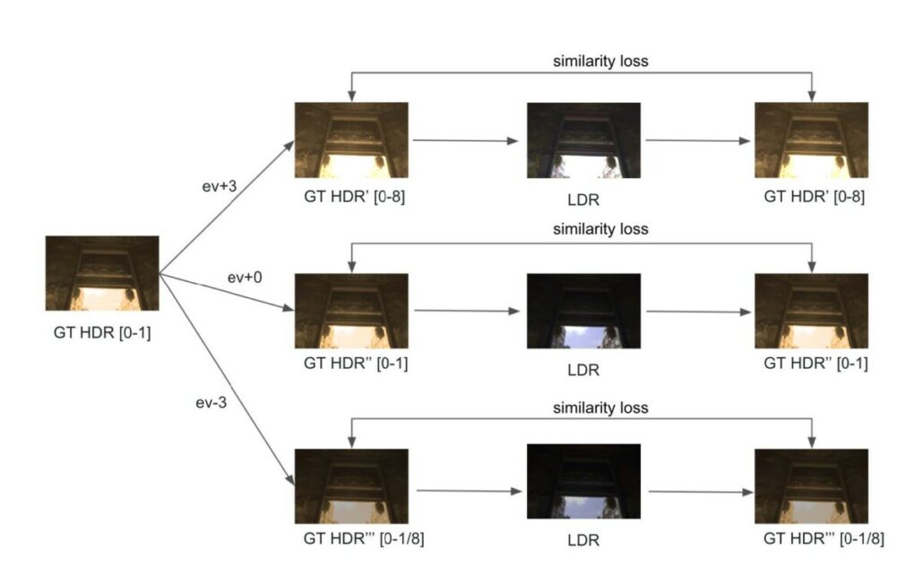
Fig. 5 our data augmentation procedure ([0-1] means 95% of pixels have values in this range).

Loss function

Our loss function is composed of  the generator loss (mean-square loss in the log domain), discriminator loss, and perceptual loss. For the perceptual loss [3], it is worth mentioning that we experiment with which layer of features to use and whether to use the features before the activation layer or after. Different VGG net layers are well-known that encode different semantic features levels, so different tasks could use different layers for perceptual loss. Features before the activation layer and the ones after the layer have different data distributions and ranges, and both have been used in different researches. In our experiments, we get the best result by using the conv3_4 layer of VGG19 before the relu activation(Fig. 6).

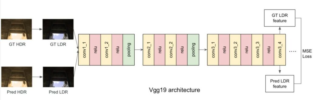
Fig. 6 The perceptual Loss.

 

Results

We show two result videos using our method. Given the image shown at the left bottom, we adjust the exposure using our model. In Video1, our method recovers the ill-exposed region on the train (see Fig. 2 to get a closer look). In Video2, we can see the contour of streetlights more clearly as we darken the image.

Video1

 

Video2